Transit is a key component of modern urban infrastructure. It contributes to the density and clustering that drive innovation and productivity - (Florida 2018)
However, many transit systems in the U.S. are not being invested into as much as systems internationally. Much of the benefits of agglomeration due to transit seem to be lost in many U.S. transit systems. Some theories as to why we don’t see the benefits from transit include a possible disconnect between house pricing and utility from transit (Bliss 2016). For instance, many people may be willing to cluster around stations but the rent premium in the area could greatly exceed the actual value added by transit. In this way, our intuitive model of supply and demand is not in equilibrium, thus making it difficult to enact policy and choose areas to implement transit. This project investigates the link between housing price and access to transit in Minneapolis, MN.
A special thanks to Dr. Sarah West who provided the house valuation data and whose research (Pilgram and West 2018) inspired this project.
1. Data Description
Our house_stop dataframe variables are outlined below:
| Variable | Meaning |
|---|---|
| address_clean | Address of the home |
| n_stops | Number of stops within a vicinity of home |
| connectivity | Number of stops accessible from stops near the home |
| mn_departures | Average number of nearby stop departures in one week |
| n_departures | mn_departures multiplied by n_stops |
| SALE_PRICE | Last price house was sold at or valuation by parcel assessor |
| SHORT_DESC | Classification of home |
| geometry | geometric identifier for simple features object |
The dataset’s 6 house SHORT_DESC or classifications in order are: Condominium, Double Bungalow, Residential, Residential Lake Shore, Townhouse, and Triplex. Because of the relative sparsity of data in the Residential Lake Shore, Townhouse, and Triplex classes, they are omitted from the analysis.
Looking at homes in Minneapolis, I want to find the transit access around a home. This is done by making a 500 m circle/buffer around each home representative of walking distance and count the number of transit stops within the buffer. It’s expected that having transit stops in the area will add to the valuation of the house.
stop_routes <- left_join(x = stops, y = as.data.frame(routes) %>% select(route_d, mn_hdwy, st_dv_h, stp_cnt))
## Warning: Column `route_d` joining factors with different levels, coercing
## to character vector

house_buffer <- st_buffer(house_sale_sf, 500) %>%
  select(one_of("address_clean", "SALE_DATE", "SALE_PRICE", "SHORT_DESC"))

house_stop_join <- st_join(x = house_buffer, y = stop_routes)
house_stop <- as.data.frame(house_stop_join) %>%
  group_by(address_clean) %>%
  summarise(
    n_stops = n(),
    connectivity = mean(stp_cnt),
    mn_departures = mean(deprtrs),
    n_departures = n_stops * mn_departures
  ) %>%
  left_join(house_buffer) %>%
  drop_na() %>%
  droplevels()

ggplot() +
  geom_sf(data = neighborhoods, color = "darkorchid4", fill = "#C6FDFF") +
  geom_sf(data = stops, color = "#E0A504", size = 0.3) +
  geom_sf(data = sample_n(house_buffer, size = 30), alpha = 0.3, fill = "#DD7373") +
  ggtitle("Transit Stops in Proximity of Addresses") +
  theme_map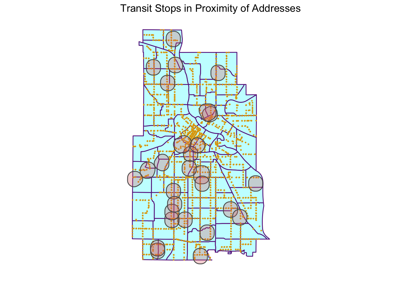
2. A Naive Model for Housing Value
Looking at the distribution of housing prices, we see a heavy right skew and apply a log transformation to normalize the distribution. Additionally looking at number of stops near a home, we see a more extreme right skew and perform the same log transformation. Plotting these logged variables shows a relatively normal distribution of logged prices conditioned on each logged n_stops.
price_dens <- ggplot(data = house_stop) +
  geom_density(mapping = aes(x = SALE_PRICE), color = "darkorchid4")
log_price_dens <- ggplot(data = house_stop) +
  geom_density(mapping = aes(x = log(SALE_PRICE)), color = "darkorchid4")
stop_dens <- ggplot(data = house_stop) +
  geom_density(mapping = aes(x = n_stops), color = "darkorchid4")
log_stop_dens <- ggplot(data = house_stop) +
  geom_density(mapping = aes(x = log(n_stops)), color = "darkorchid4")

grid.arrange(price_dens, log_price_dens, stop_dens, log_stop_dens, ncol=2)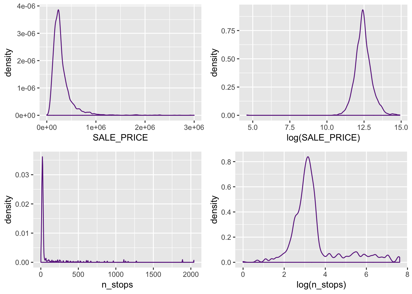
ggplot(data = house_stop %>% filter(log(SALE_PRICE) > 10), (mapping = aes(x = log(n_stops), y = log(SALE_PRICE)))) +
  geom_point(color = "darkorchid4")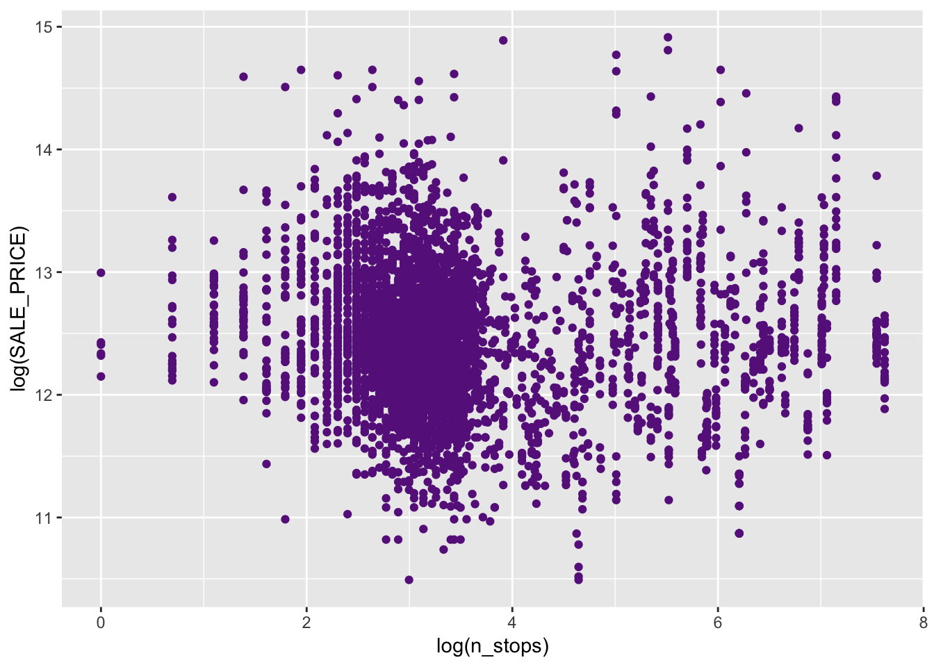
I begin by estimating a Bayesian normal-normal model for the specification below. For house \(i\), let \(Y_i\) be the valuation, \(S_i\) be the number of stops within 500 meters, and \(T_{ij}\) be a binary categorical variable for the type \(j\) of the house. A log specification is put on the price and number of stops to normalize the variables.
\[\begin{align*} \displaystyle \ln{Y_i}|\beta_0, \beta_1, \tau &\sim N\left(\ \beta_0 + \beta_1 \ln{S_i} + \sum_{j = 1}^{3}T_{ij} \ , \; \tau^{-1} \ \right) \\ \beta_0 &\sim N(10^4 \ , \ 10^6) \\ \beta_1 &\sim N(50 \ , \ 10^6) \\ T_{j} &\sim N(0\ ,\ 10^6) \\ \tau &\sim Gamma(100, 3000) \end{align*}\]#Collect Model Prior Parameters and Data
data_th1 <- list(price = log(house_stop$SALE_PRICE), stops = log(house_stop$n_stops), type = factor(house_stop$SHORT_DESC))
model_th1 <-
"
model{
# Regression Response
for(i in 1:length(price)) {
price[i] ~ dnorm(mu[i], tau)
mu[i] <- beta_0 + beta_1 * stops[i] + beta_t[type[i]]
}
# Parameters
beta_0 ~ dnorm(10000, 1e-6)
beta_1 ~ dnorm(50, 1e-6)
beta_t[1] <- 0
for(cat in 2:3) {
beta_t[cat] ~ dnorm(0, 1e-6)
}
tau ~ dgamma(100, 3000)
}
"
#Compile Model
jags_th1 <- jags.model(
file = textConnection(model_th1),
data = c(data_th1),
inits = list(.RNG.name = "base::Wichmann-Hill", .RNG.seed = 454),
quiet = TRUE
)
# Burn in 1000 iterations
update(jags_th1, 1000, progress.bar = "none")
#Sample from Markov Chain
sim_th1 <- coda.samples(
model = jags_th1,
variable.names = c("beta_0", "beta_1", "beta_t", "tau"),
n.iter = 10000
)
summary(sim_th1)
##
## Iterations = 1001:11000
## Thinning interval = 1
## Number of chains = 1
## Sample size per chain = 10000
##
## 1. Empirical mean and standard deviation for each variable,
## plus standard error of the mean:
##
## Mean SD Naive SE Time-series SE
## beta_0 12.42424 0.11396 0.0011396 0.0095922
## beta_1 -0.00208 0.02124 0.0002124 0.0016454
## beta_t[1] 0.00000 0.00000 0.0000000 0.0000000
## beta_t[2] 0.13089 0.07560 0.0007560 0.0039566
## beta_t[3] 0.02570 0.06149 0.0006149 0.0042166
## tau 0.67740 0.01342 0.0001342 0.0001365
##
## 2. Quantiles for each variable:
##
## 2.5% 25% 50% 75% 97.5%
## beta_0 12.21088 12.34803 12.419298 12.49933 12.65112
## beta_1 -0.04341 -0.01598 -0.001368 0.01219 0.03796
## beta_t[1] 0.00000 0.00000 0.000000 0.00000 0.00000
## beta_t[2] -0.02165 0.08085 0.131864 0.18245 0.27523
## beta_t[3] -0.09747 -0.01636 0.028022 0.06755 0.14096
## tau 0.65139 0.66826 0.677115 0.68635 0.70408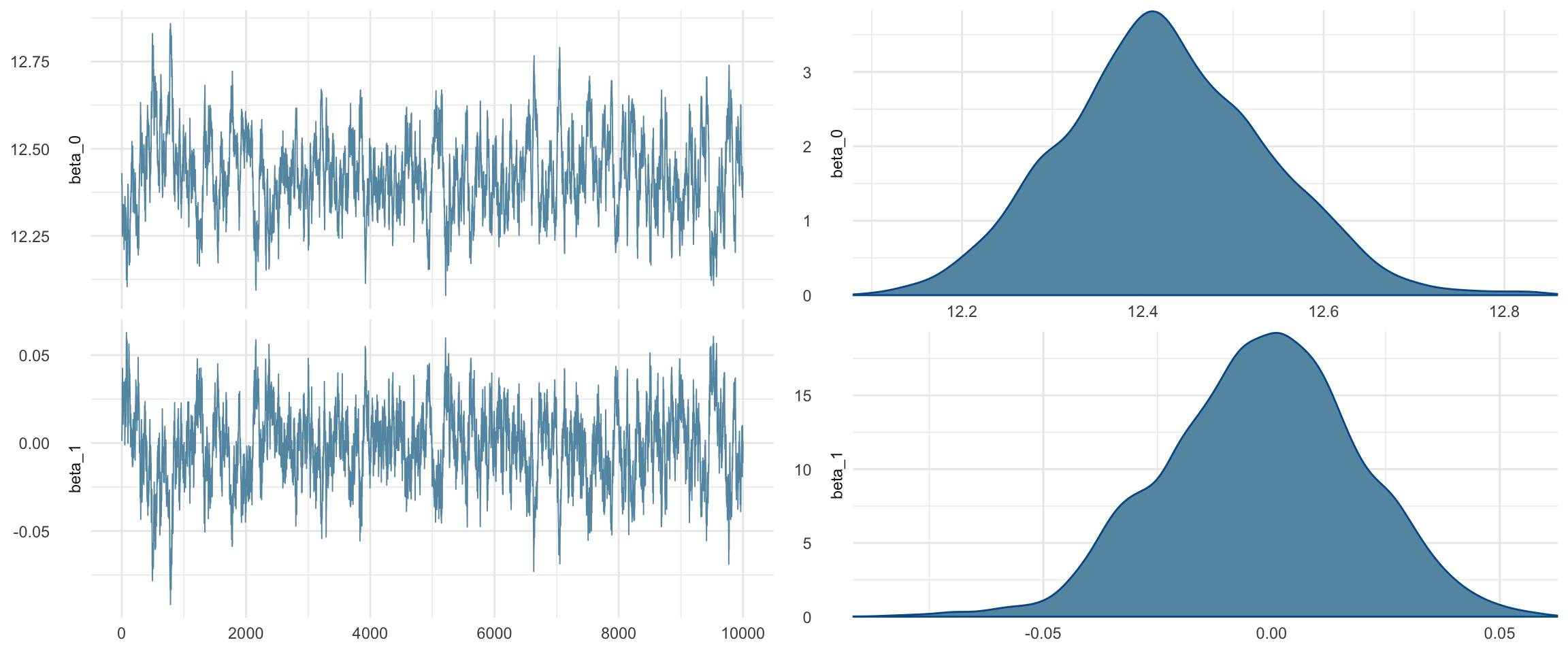
This model can be interpreted in terms of percentage changes due to the logged price response and logged number of stops predictor. Surprisingly, the model tells us that number of transit stops negatively affects the house price. More precisely, a %10 increase in number of stops decreases the home price by about %2.53. This model is a great place to start in evaluating transit value but it’s definitely not the best we can do. Spatial data is known for high levels of spatial autocorrelation. In other words, houses in the same general location will have similar prices. While this will not be addressed in this research, it is something to consider moving forward.
More pressing is that we haven’t distinguished between different stops and their contribution to a measure of transit access. We are treating a low frequency bus stop in the suburbs the same as a high frequency downtown light rail stop. We will attempt to address these by specifying data features which capture the frequency and connectedness of each stop.
3. Implementing the Stop Characteristics
In this next section I want to iterate on the previous model towards a better specification incorporating more information from each stop. I also notice that among each group, the relationship between valuation and transit access varies.
departure_price <-ggplot(data = house_stop %>% filter(log(SALE_PRICE) > 10), mapping = aes(x = log(n_departures), y = log(SALE_PRICE))) +
  geom_point(color = "darkorchid4") +
  geom_smooth(method='lm', se = FALSE, color = "#E0A504") +
  facet_wrap(facets = vars(SHORT_DESC))

connect_price <- ggplot(data = house_stop %>% filter(log(SALE_PRICE) > 10, log(connectivity) > 4), mapping = aes(x = log(connectivity), y = log(SALE_PRICE))) +
  geom_point(color = "darkorchid4") +
  geom_smooth(method='lm', se = FALSE, color = "#E0A504") +
  facet_wrap(facets = vars(SHORT_DESC))

grid.arrange(departure_price, connect_price, nrow=2)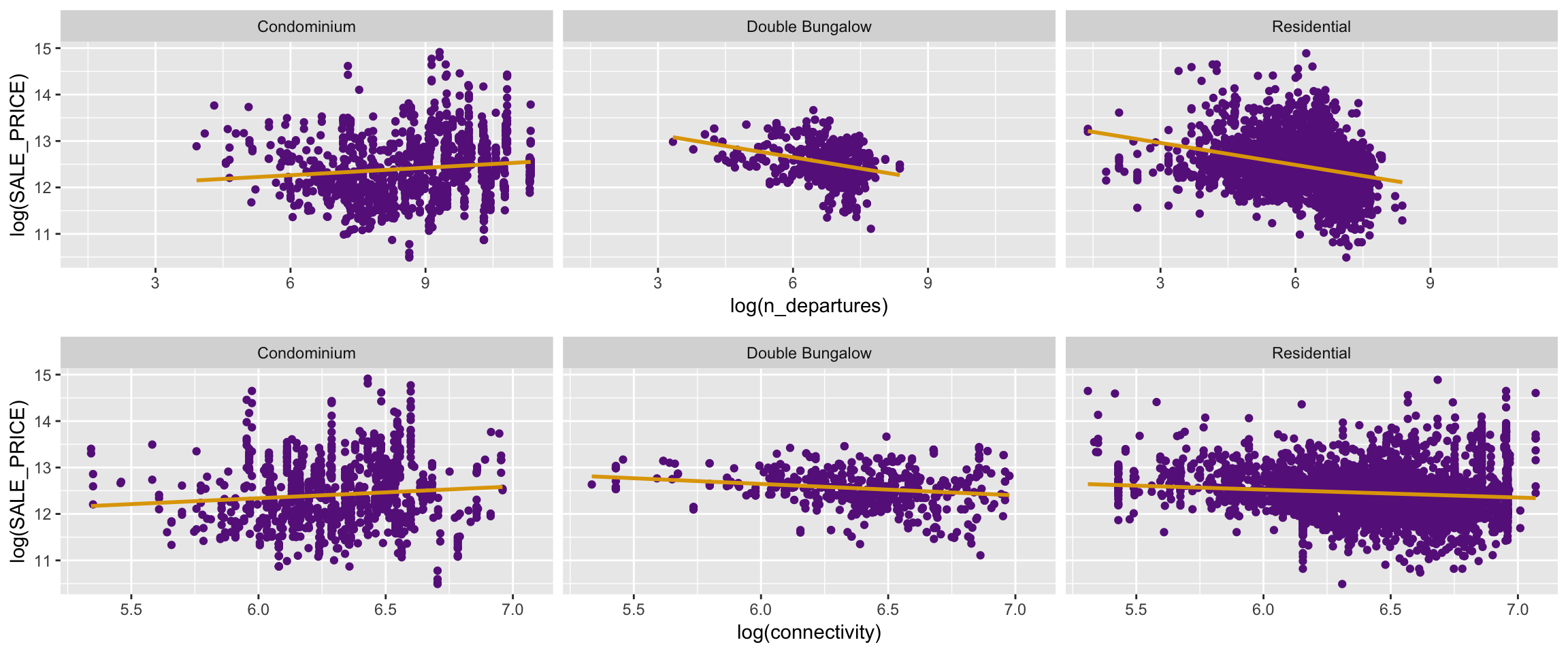
To better understand the utility of a stop, instead of looking at the number of stops, I looked at the number of weekly arrivals at that stop and summed up for all stops in the vicinity of a house. In other words, the number of weekly transit arrivals near a house, \(i\), represented by \(D_i\). Similar to what was done in the previous model, I apply a log transformation to departures and connectivity. For this model, we want to capture the individual house price trend for each house group with respect to our covariates. This is known as mixed effects, where there’s a different set of slopes and coefficients for each group, which in our case is house type \(j\).
\[\begin{align*} \displaystyle \ln{Y_{ij}} | b_{0j}, b_{1j}, b_{2j} \tau_w &\sim N\left(\ b_{0j} + b_{1j} \ln{D_{ij}} + b_{2j} \ln{C_{ij}}\ , \; \tau_w^{-1} \ \right) \\ b_{0j} | \beta_0, \tau_{0b} &\sim N(\beta_0, \tau_{0b}) \\ b_{1j} | \beta_1, \tau_{1b} &\sim N(\beta_1, \tau_{1b}) \\ b_{2j} | \beta_2, \tau_{2b} &\sim N(\beta_2, \tau_{2b}) \\ \beta_0 &\sim N(10^4, 10^6) \\ \beta_1, \beta_2 &\sim N(50, 10^6) \\ \tau_w, \tau_{0b}, \tau_{1b}, \tau_{2b} &\sim Gamma(100, 3000) \end{align*}\]#Collect Model Prior Parameters and Data
data_th2 <- list(price = log(house_stop$SALE_PRICE), type = factor(house_stop$SHORT_DESC), departures = log(house_stop$n_departures), connectivity = log(house_stop$connectivity))
model_th2 <-
"
model{
# Regression Response
for(i in 1:length(price)) {
price[i] ~ dnorm(b0[type[i]] + b1[type[i]]*departures[i] + b2[type[i]]*connectivity[i], tauw)
}
# Parameters
for(cat in 1:3) {
b0[cat] ~ dnorm(beta_0, tau0b)
b1[cat] ~ dnorm(beta_1, tau1b)
b2[cat] ~ dnorm(beta_2, tau2b)
}
beta_0 ~ dnorm(10000, 1e-6)
beta_1 ~ dnorm(50, 1e-6)
beta_2 ~ dnorm(50, 1e-6)
tauw ~ dgamma(100, 3000)
tau0b ~ dgamma(100, 3000)
tau1b ~ dgamma(100, 3000)
tau2b ~ dgamma(100, 3000)
}
"
#Compile Model
jags_th2 <- jags.model(
file = textConnection(model_th2),
data = c(data_th2),
inits = list(.RNG.name = "base::Wichmann-Hill", .RNG.seed = 454)
)
## Compiling model graph
## Resolving undeclared variables
## Allocating nodes
## Graph information:
## Observed stochastic nodes: 4945
## Unobserved stochastic nodes: 16
## Total graph size: 26009
##
## Initializing model
# Burn in 1500 iterations
update(jags_th2, 2000, progress.bar = "none")
#Sample from Markov Chain
sim_th2 <- coda.samples(
model = jags_th2,
variable.names = c("b0", "b1", "b2", "beta_0", "beta_1", "beta_2", "tauw", "tau0b", "tau1b", "tau2b"),
n.iter = 10000
)
summary(sim_th2)
##
## Iterations = 2001:12000
## Thinning interval = 1
## Number of chains = 1
## Sample size per chain = 10000
##
## 1. Empirical mean and standard deviation for each variable,
## plus standard error of the mean:
##
## Mean SD Naive SE Time-series SE
## b0[1] 9.13489 2.725145 2.725e-02 8.934e-01
## b0[2] 14.18394 1.331458 1.331e-02 4.208e-01
## b0[3] 14.00642 0.414641 4.146e-03 9.721e-02
## b1[1] 0.05781 0.023879 2.388e-04 2.127e-03
## b1[2] -0.14514 0.068292 6.829e-04 8.571e-03
## b1[3] -0.16044 0.022003 2.200e-04 2.022e-03
## b2[1] 0.43935 0.427225 4.272e-03 1.386e-01
## b2[2] -0.10521 0.214757 2.148e-03 6.792e-02
## b2[3] -0.08729 0.065639 6.564e-04 1.551e-02
## beta_0 12.51711 3.451428 3.451e-02 2.019e-01
## beta_1 -0.09308 3.120552 3.121e-02 3.121e-02
## beta_2 0.05775 3.181418 3.181e-02 3.147e-02
## tau0b 0.03351 0.003310 3.310e-05 3.439e-05
## tau1b 0.03364 0.003353 3.353e-05 3.353e-05
## tau2b 0.03367 0.003321 3.321e-05 3.321e-05
## tauw 0.68520 0.014743 1.474e-04 9.270e-04
##
## 2. Quantiles for each variable:
##
## 2.5% 25% 50% 75% 97.5%
## b0[1] -0.76495 9.09248 9.94029 10.47242 11.29739
## b0[2] 10.30328 13.37364 14.25437 15.10662 16.33110
## b0[3] 12.87712 13.78603 14.05549 14.27994 14.65720
## b1[1] 0.01082 0.04154 0.05804 0.07441 0.10355
## b1[2] -0.28684 -0.19057 -0.13861 -0.09619 -0.02423
## b1[3] -0.20466 -0.17534 -0.16005 -0.14470 -0.11981
## b2[1] 0.09535 0.23116 0.31614 0.44780 1.98976
## b2[2] -0.47135 -0.25850 -0.10584 0.02749 0.45175
## b2[3] -0.18998 -0.12960 -0.09371 -0.05230 0.09778
## beta_0 5.45126 10.27234 12.57154 14.86862 19.04893
## beta_1 -6.24677 -2.21464 -0.07631 2.01801 5.88447
## beta_2 -6.26409 -2.09940 0.08820 2.17931 6.29058
## tau0b 0.02731 0.03122 0.03340 0.03565 0.04025
## tau1b 0.02744 0.03130 0.03348 0.03586 0.04053
## tau2b 0.02745 0.03136 0.03360 0.03587 0.04048
## tauw 0.65445 0.67592 0.68559 0.69486 0.71333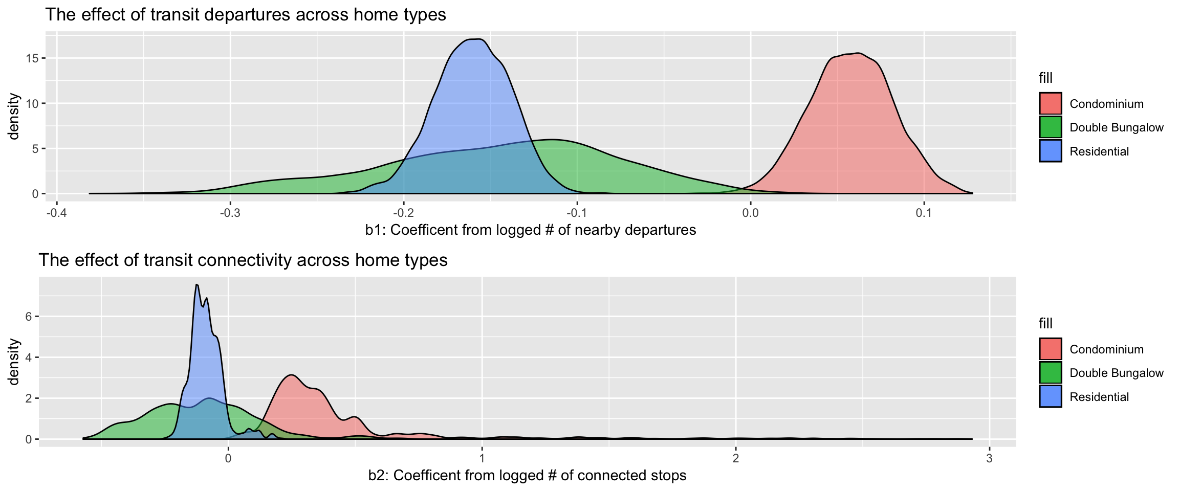
Our model says that condos tend to be the houses where both transit frequency and connectivity increase the valuation the most consistently. Whereas residential classified homes seem to have their prices decreased by the two transit factors. The double bungalow class seems to be an intermediate with both more variant and closer to 0 price effect from transit activity.
4. Predicting House Price
To test out our model let’s try to predict a house’s price. Looking at some hypothetical house, we want to predict how much any condominium would cost if there’s around 3000 departures per week and around 600 stops its connected to. This is decently reasonable given the mean and median for departures and connectivity.
pred_chains_th2 <- chains_th2 %>%
  mutate(
    predict_ln = rnorm(n = n(), mean = (b0.1. + b1.1. * log(3000) + b2.1. * log(500)), sd = sqrt(1/tauw)),
    predict = exp(predict_ln)
  )

ggplot(data = pred_chains_th2) +
  geom_density(mapping = aes(x = predict_ln), color = "darkorchid4") +
  geom_vline(mapping = aes(xintercept = mean(pred_chains_th2$predict_ln)), color = "#E0A504")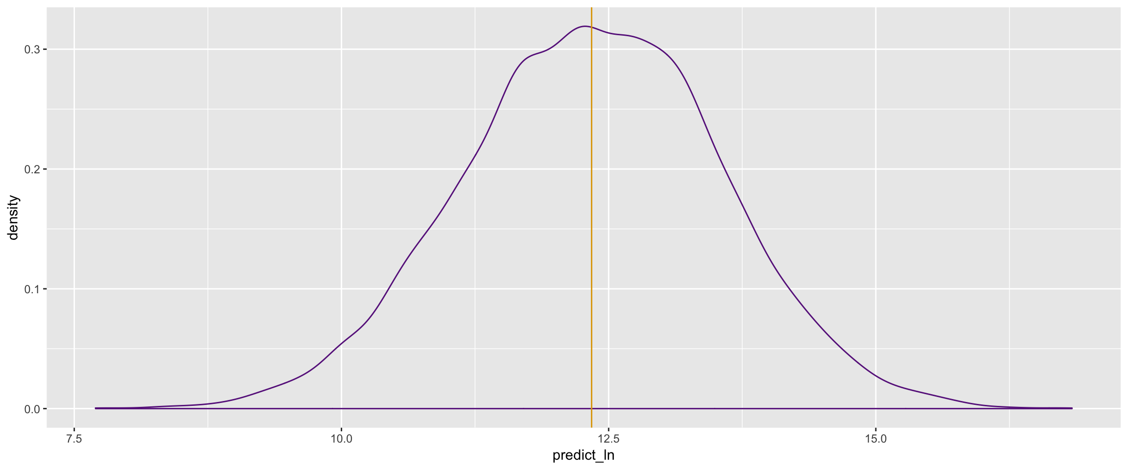
mean(pred_chains_th2$predict_ln)
## [1] 12.34057
exp(mean(pred_chains_th2$predict_ln))
## [1] 228792.1
From the logged posterior predictive distribution above, we exponentiate the mean to find the expected price of a residential home with 3000 nearby departures per week and 500 connected stops to be about $230,000.
5. Closing Thoughts
In this study, I looked at the effect of transit activity near a home on its valuation. Controlling for the type of the home and splitting up transit activity into the number of weekly departures and the connectivity of the stop. Among the 3 classes of houses, I find mixed effects from both predictors. Condos tend to have their prices increased consistently by transit, residential homes consistently have their prices decreased, and double bungalows are more variant but generally have little to no transit price premiums.
In the future, I’d like to think a little bit more about how I can classify access to transit from a home. For instance, a stop may be within a walking distance radius but may still be difficult to get to. Furthermore, I haven’t yet controlled for other key distinctions which are main drivers in housing price such as number of rooms or value of construction. Simply put, my model has not yet put in the necessary controls to isolate the value of transit. A possible thought project I had wanted to explore is the scenario of a highly valuated and or upcoming neighborhood likely to have new residents and evaluate whether the transit access in that area is fit to handle the influx of new population/activity. Finally, we still haven’t addressed the idea of spatial autocorrelation and similarity between neighbors. In a follow up, I’d like to apply an inverse distance weighting for the information provided by each data to account for spatial autocorrelation and possibly control for other home assets.
References
Bliss, Laura. 2016. “The Tricky Relationship Between Transit and Land Value.” CityLab. https://www.citylab.com/transportation/2016/04/transit-station-property-value-study/479730/.
Florida, Richard. 2018. “The Global Mass Transit Revolution.” CityLab. https://www.citylab.com/transportation/2018/09/the-global-mass-transit-revolution/570883/.
Pilgram, Clemens A., and Sarah E. West. 2018. “Fading Premiums: The Effect of Light Rail on Residential Property Values in Minneapolis, Minnesota.” Regional Science and Urban Economics 69: 1–10. doi:https://doi.org/10.1016/j.regsciurbeco.2017.12.008.