A Tutorial on Non-Parametric Kernel Density Estimation

Apr 19, 2019 9 min read R

1. Introduction

Nonparametric statistics is a field that has been rapidly developing over the last decade. Its development has been aided by the various benefits it has relative to classical statistical techniques:

We can relax assumptions on the probability distribution of the data. Most notably, the normality.
There are cases in which classical procedures are neither applicable nor interpretable but a nonparametric one is.
Modern computing has empowered many of these computationally expensive techniques.

So far, when approaching statistics problems, we’ve assumed the distribution of data. However, we rarely ever understand the data enough to confidently assume a distribution. We will cover Kernel Density Estimation (KDE), a non-parametric estimation technique for any distribution f(x). We will start with an explanation and mathematical form of a kernel density estimator, go over its properties, and touch on the burgeoning field of bandwidth selection.

2. History

The concept of KDE was created by Parzen (1962) and Rosenblatt (1956) in their independent works, so it is also called Parzen-Rosenblatt window method in other fields such as signal processing and econometrics.

3. Some Intuition

The Histogram

Non-parametric density estimation may sound very alien but in fact it’s so commonplace that we’ve already seen it countless times! In high school, and even earlier, we’ve come across the $histogram$ . Turns out, they are non-parametric density estimators.

We split our data into into $K$ equally sized bins/intervals with boundaries $a_{0}, a_{1}, \dots, a_{K}$ and estimate the density in bin i as the proportion of observations that fall within $(a_{i - 1}, a_{i}]$ . Let $n_{i}$ be the number of observations within interval $(a_{i - 1}, a_{i}]$ and $K$ be the number of bins, for a histogram from distribution $X$ with sample size $N$ :

\hat{f} (s) = \frac{1}{N} \sum_{i = 0}^{K - 1} \frac{n_{i}}{a_{i} - a_{i - 1}} I_{(a_{i - 1}, a_{i}]} (s)

However, there are problems with this. First, histograms tend to be blocky and sensitive to bins chosen.

some_data <- rchisq(n = 100, df = 5)
hist_bins <- function(data, bins) {
  ggplot(mapping = aes(x = data, y=..density..)) +
  geom_histogram(bins = bins, fill = "darkorchid4") + 
  ggtitle(sprintf(fmt = "%i bins", bins))
}

grid.arrange(hist_bins(some_data, 10), 
             hist_bins(some_data, 20), 
             hist_bins(some_data, 40), 
             hist_bins(some_data, 80), nrow=2)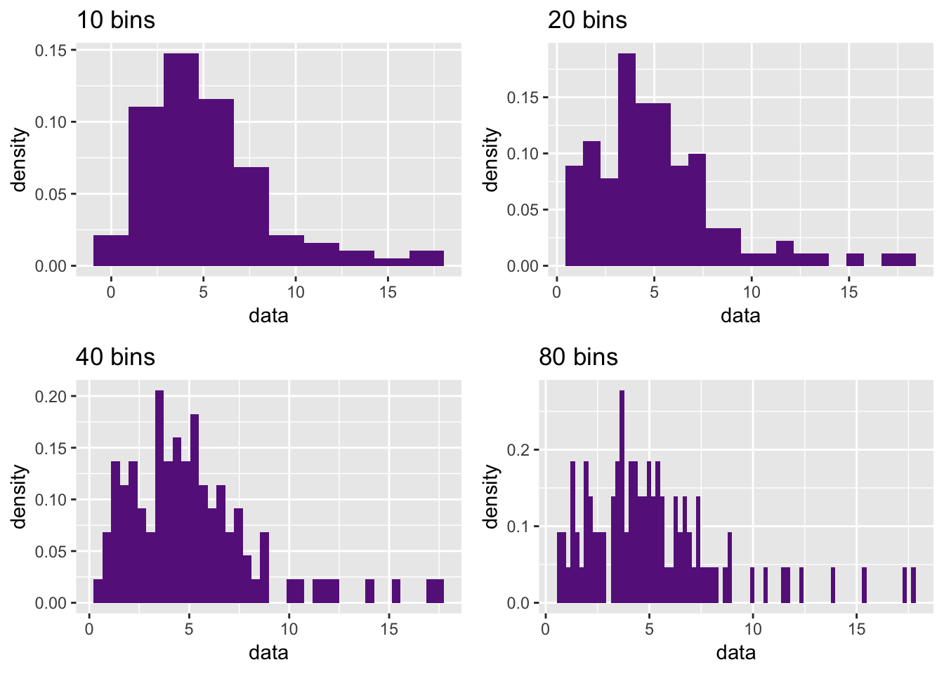Show Source

Also, histograms are inherently local; I can have an observation $x = 4.99999$ not counted in interval $[5, 6]$ .

Kernel Density Estimation

A kernel density estimate, ${\hat{f}}_{N} (s)$ , looks at some some point $s$ and the window $[s - h / 2, s + h / 2]$ , where $h$ is chosen bandwith, and counts the observations in the window.

\begin{aligned} {\hat{f}}_{N} (s) & = \frac{1}{N} \sum_{i = 1}^{N} \frac{1}{h} I_{[s - h / 2, s + h / 2]} (X_{i}) = \frac{1}{N h} \sum_{i = 1}^{N} I_{[- h / 2, h / 2]} (X_{i} - s) \\ = \frac{1}{N h} \sum_{i = 1}^{N} I_{[- 1 / 2, 1 / 2]} (\frac{X_{i} - s}{h}) \end{aligned}

We transform the initial equation with $X_{i}$ into a “distance” of surrounding X_i away from our point of interest s weighted by bandwidth, $\frac{X_{i} - s}{h}$ . Thus, instead of fixed bins, we have a moving window and can weigh $x = 4.99999$ accurately. However the roughness remains due to weighing each point in the window equally. You can think of a kernel function as a weighting function. Now, instead of weighing all distances from $s$ the same, we can apply a smooth kernel function such as a Gaussian (normal) function which will weight smaller distances more and larger distances less towards the density at $s$ .

{\hat{f}}_{N} (x) = \frac{1}{N h} \sum_{i = 1}^{N} K (\frac{x - X_{i}}{h})

Above, $K$ is our kernel/weighting function. The gaussian kernel function is very apparent in this low bandwidth ( $h = 0.3$ ) computation below. We look at a $N = 100$ sample from Binom $(100, 0.5)$ .

binom_data <- rbinom(n = 10000, size = 20, prob = 0.5)
ggplot(mapping = aes(x = binom_data)) +
  geom_histogram(mapping = aes(y = ..density..), bins = 10, fill = "darkorchid4") + 
  geom_density(kernel = "gaussian", bw = 0.3, color = "#d2bf55", size = 1)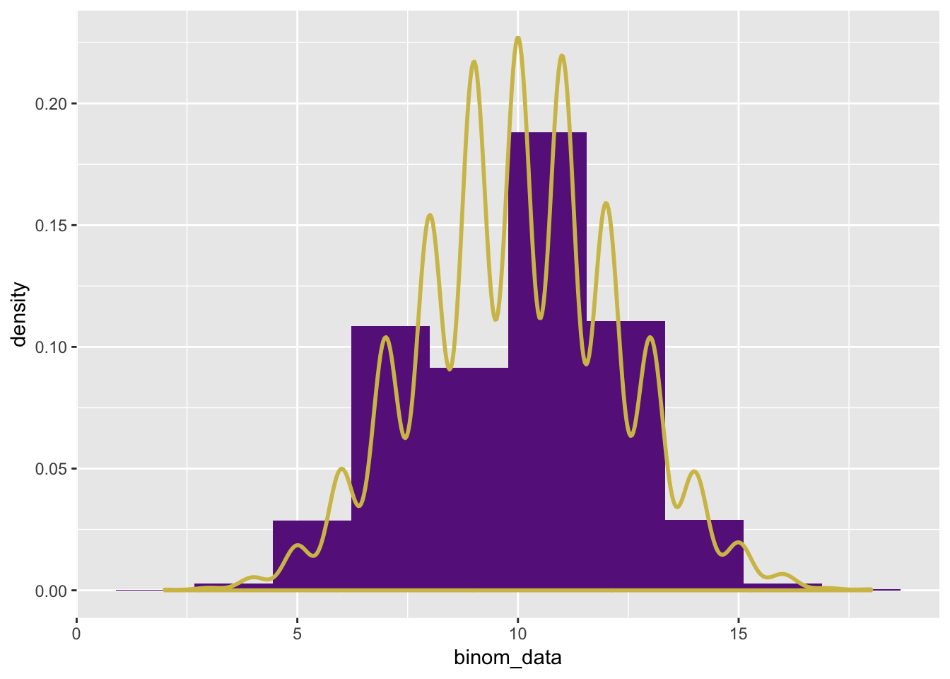Show Source

4. Theory and Properties

To allow for our analysis of KDE properties, we will outline a few rules about the Kernel and underlying density function.

Kernel function $K$ : is symmetric about 0, $\int_{Ω_{X}} K d x = 1$ , and $lim_{x \to - \infty} K (x) = lim_{x \to \infty} K (x) = 0$
$\int x K (x) d x < \infty$ and $\int | x | (K (x))^{2} d x < \infty$
PDF $f$ : $R \to R$ is Lipschitz Continuous, $\exists M \in R, | f (x) - f (y) | \leq M | x - y |, \forall x, y \in R$

Applications of assumptions will be notated in brackets (i.e: [1]). Proof is adapted from Wasserman (2006) and simplified.

Bias

As with most estimators, we want to account for bias. For $X_{1}, X_{2}, \dots, X_{N} \overset{i i d}{\sim} f$ , the expected value of the kernel density estimate at $s$ : $E [{\hat{f}}_{N} (s)] = E [\frac{1}{N h} \sum_{i = 1}^{N} K (\frac{X_{i} - s}{h})] = \frac{1}{h} E [K (\frac{X - s}{h})] = \frac{1}{h} \int K (\frac{x - s}{h}) f (x) d x$ We set $u = \frac{x - s}{h}$ , substitute, and apply a $2^{n d}$ order Taylor series expansion for $f (h u + s)$ about $h = 0$ :

\begin{aligned} E [{\hat{f}}_{N} (s)] & = \frac{1}{h} \int K (u) f (h u + s) h d u = \int K (u) f (h u + s) d u \\ f (h u + s) & = f (s) + \frac{f^{'} (s)}{1!} (u) (h - 0) + \frac{f^{″} (s)}{2!} (u^{2}) (h - 0)^{2} + o (h^{2}) \\ = f (s) + h u f^{'} (s) + \frac{h^{2} u^{2}}{2} f^{″} (s) + o (h^{2}) \end{aligned}

$o (h^{2})$ is some function that as $h \to 0$ , $o (h^{2}) \to 0$ is negligible compared to $h^{2}$ . Plugging in our Taylor approximation for $f (h u + s)$ :

\begin{aligned} E [{\hat{f}}_{N} (s)] & = \int K (u) [f (s) + h u f^{'} (s) + \frac{h^{2} u^{2}}{2} f^{″} (s) + o (h^{2})] d u \\ = f (s) \underset{[1], = 1}{\underset{⏟}{\int K (u) d u}} + h f^{'} (s) \underset{[1], = 0}{\underset{⏟}{\int u K (u) d u}} + \frac{h^{2}}{2} f^{″} (s) \int u^{2} K (u) d u + o (h^{2}) \\ = f (s) + \frac{h^{2}}{2} f^{″} (s) \int u^{2} K (u) d u + o (h^{2}), Thus... \\ Bias ({\hat{f}}_{N} (s)) & = E [{\hat{f}}_{N} (s)] - f (s) = \frac{h^{2}}{2} f^{″} (s) \underset{constant}{\underset{⏟}{\int u^{2} K (u) d u}} + \underset{bounded}{\underset{⏟}{o (h^{2})}} \\ = \frac{t \cdot h^{2}}{2} f^{″} (s) + o (h^{2}), t = \int u^{2} K (u) d u \end{aligned}

From this we can see that the lower bandwidth $h$ we choose, the less bias we get. We also get the inisght that bias is highest at points $s$ where the curvature is very high, such as at a sharp peak. This is pretty apparent when we think of high KDE tries to smooth around these rough edges in the data.

Variance

Similarly, we find the upper bound for variance of estimated density, ${\hat{f}}_{N}$ at some point $s$ :

\begin{aligned} V a r ({\hat{f}}_{N} (s)) & = V a r (\frac{1}{N h} \sum_{i = 1}^{N} K (\frac{X_{i} - s}{h})) \\ = \frac{1}{N h^{2}} (E [K^{2} (\frac{X - s}{h})] - E {[K (\frac{X - s}{h})]}^{2}), K is symmetric about s [1] \\ \leq \frac{1}{N h^{2}} E [K^{2} (\frac{X - s}{h})] \\ = \frac{1}{N h^{2}} \int K^{2} (\frac{x - s}{h}) f (x) d x \end{aligned}

We now substitute $u = \frac{x - s}{h}$ and approximate $f (h u + s)$ via $1^{s t}$ order Taylor series expansion about $h = 0$ :

\begin{aligned} V a r ({\hat{f}}_{N} (s)) & \leq \frac{1}{N h^{2}} \int K^{2} (u) f (h u + s) h d u \\ = \frac{1}{N h} \int K^{2} (u) f (h u + s) d u \\ = \frac{1}{N h} \int K^{2} (u) [f (s) + h u f^{'} (s) + o (h)] d u \\ = \frac{1}{N h} (f (s) \int K^{2} (u) d u + h f^{'} (s) \underset{[1], = 0}{\underset{⏟}{\int u K^{2} (u) d u}} + o (h)) \\ V a r ({\hat{f}}_{N} (s)) & \leq \frac{f (s)}{N h} \underset{constant}{\underset{⏟}{\int K^{2} (u) d u}} + \underset{bounded}{\underset{⏟}{o (\frac{1}{N h})}} \\ = \frac{z}{N h} f (s) + o (\frac{1}{N h}), z = \int K^{2} (u) d u \end{aligned}

Because $\frac{1}{N h}$ is the other function of $h$ in this expression, we say that as $h \to 0$ and $N \to \infty$ , $o (\frac{1}{N h})$ is some function that is negligible compared to $\frac{1}{N h}$ . We observe that the variance of our kernel density estimate $V a r ({\hat{f}}_{N} (s))$ is high at points of high density in the true distribution, $f (s)$ . We also see that increasing either sample size or bandwidth decreases this upper bound.

Bringing it Together: MSE

Knowing both bias and variance of KDE predictors, it’s natural to look towards computing the Mean Squared Error (MSE).

\begin{aligned} MSE ({\hat{f}}_{N} (s)) & = {Bias}^{2} ({\hat{f}}_{N} (s)) + Var ({\hat{f}}_{N} (s)) \\ = {(\frac{t h^{2}}{2} f^{″} (s) + o (h^{2}))}^{2} + \frac{z}{N h} f (s) + o (\frac{1}{N h}); t = \int u^{2} K (u) d u, z = \int K^{2} (u) d u \\ = \frac{t^{2} h^{4}}{4} {[f^{″} (s)]}^{2} + \frac{z}{N h} f (s) + o (h^{4}) + o (\frac{1}{N h}) \end{aligned}

The Mean Squared Error can be treated as a risk function similar to what we saw in Bayesian predictors. $\frac{t^{2} h^{4}}{4} {[f^{″} (s)]}^{2} + \frac{z}{N h} f (s)$ is the $Asymptotic Mean Squared Error (AMSE)$ . With this it’s quite straightforward to optimize with respect to $h$ .

\begin{aligned} \frac{\partial}{\partial h} AMSE ({\hat{f}}_{N} (s)) & = \frac{\partial}{\partial h} (\frac{t^{2}}{4} {[f^{″} (s)]}^{2}) h^{4} + (\frac{z}{N} f (s)) \frac{1}{h} \\ = (t^{2} {[f^{″} (s)]}^{2}) h^{3} - (\frac{z}{N} f (s)) \frac{1}{h^{2}} \\ 0 & = (t^{2} {[f^{″} (s)]}^{2}) h^{5} - (\frac{z}{N} f (s)) \\ h_{o p t} & = {(\frac{z f (s)}{N t^{2} {[f^{″} (s)]}^{2}})}^{\frac{1}{5}} = C_{1} N^{- \frac{1}{5}} \end{aligned}

5. Choosing Bandwidth

Bandwidth is similar to bin width in histograms. Bandwidth determines how smooth the KDE curves can be. If the chosen bandwidth is very small, the curve will be high variance; this case is called undersmoothing. If the chosen bandwidth is too large, however, the curve will have high bias and we are oversmoothing the curve.

Because an appropriate size of bandwidth yields optimal results of estimation, bandwidth selection is a very important topic. If we choose a correct bandwidth, we will be able to estimate the underlying distribution, which neither wiggles too much (with a very small bandwidth) nor loses its characteristics (with a very large bandwidth).

Although there are many different bandwidth selection methods, the main idea of these methods is to minimize the asymptotic mean integrated square error (AMISE). You might’ve thought that we’ve already found the optimal $h$ , but previously we only found the $h_{o p t}$ for a single point $s$ . To do this for the entire distribution we must optimize on the same AMSE just integral along all value of the distribution. We provide the tools below and leave this as a simple exercise for the reader:

$MISE ({\hat{f}}_{N} (s)) = \underset{AMISE ({\hat{f}}_{N} (s))}{\underset{⏟}{\int (\frac{t^{2} h^{4}}{4} {[f^{″} (s)]}^{2} + \frac{z}{N h} f (s)) d x}} + o (\frac{1}{N h})$

In the end, you should find $h_{o p t}$ is dependent on the overall curvature of the underlying distribution $\int {[f^{″} (x)]}^{2} d x$ . Despite the age of the KDE concept, many of the advances in KDE are within the last decade in the field of bandwidth selection. If you find a good way to estimate $AMISE$ or the overall curvature, $\int {[f^{″} (x)]}^{2} d x$ , prepare to get published. See Wang and Zambom (2019) and Goldenshluger, Lepski, and others (2011).

References

Goldenshluger, Alexander, Oleg Lepski, and others. 2011. “Bandwidth Selection in Kernel Density Estimation: Oracle Inequalities and Adaptive Minimax Optimality.” The Annals of Statistics 39 (3). Institute of Mathematical Statistics: 1608–32.

Parzen, Emanuel. 1962. “On Estimation of a Probability Density Function and Mode.” The Annals of Mathematical Statistics 33 (3). JSTOR: 1065–76.

Rosenblatt, Murray. 1956. “Remarks on Some Nonparametric Estimates of a Density Function.” The Annals of Mathematical Statistics. JSTOR, 832–37.

Wang, Qing, and Adriano Z Zambom. 2019. “Subsampling-Extrapolation Bandwidth Selection in Bivariate Kernel Density Estimation.” Journal of Statistical Computation and Simulation. Taylor & Francis, 1–20.

Wasserman, Larry. 2006. All of Nonparametric Statistics. Springer Science & Business Media.